Overview

This post outlines how to use the teamlucc package to filter the Landsat imagery available in the archives for a particular study site. teamlucc includes several functions to make plots to assist with selecting anniversary dates (or near anniversary dates…) when multiple Landsat path/rows are needed to cover a single site. The teamlucc package also has functions to output an order text file in the proper format for the USGS ESPA system and to automatically download and verify the completed portions of a USGS ESPA order.

Getting started

First load the devtools package, used for installing teamlucc. Install the devtools package if it is not already installed:

if (!require(devtools)) install.packages('devtools')

Now load the teamlucc package, using devtools to install it from github if it is not yet installed. Also load the rgdal package needed for reading/writing shapefiles:

if (!require(teamlucc)) install_github('azvoleff/teamlucc')

## Loading required package: teamlucc
## Loading required package: Rcpp
## Loading required package: raster
## Loading required package: sp

## Warning: replacing previous import by 'raster::buffer' when loading
## 'teamlucc'

## Warning: replacing previous import by 'raster::interpolate' when loading
## 'teamlucc'

## Warning: replacing previous import by 'raster::rotated' when loading
## 'teamlucc'

library(rgdal)

## rgdal: version: 0.9-1, (SVN revision 518)
## Geospatial Data Abstraction Library extensions to R successfully loaded
## Loaded GDAL runtime: GDAL 1.11.0, released 2014/04/16
## Path to GDAL shared files: C:/Users/azvoleff/R/win-library/3.1/rgdal/gdal
## GDAL does not use iconv for recoding strings.
## Loaded PROJ.4 runtime: Rel. 4.8.0, 6 March 2012, [PJ_VERSION: 480]
## Path to PROJ.4 shared files: C:/Users/azvoleff/R/win-library/3.1/rgdal/proj

Downloading list of available Landsat scenes

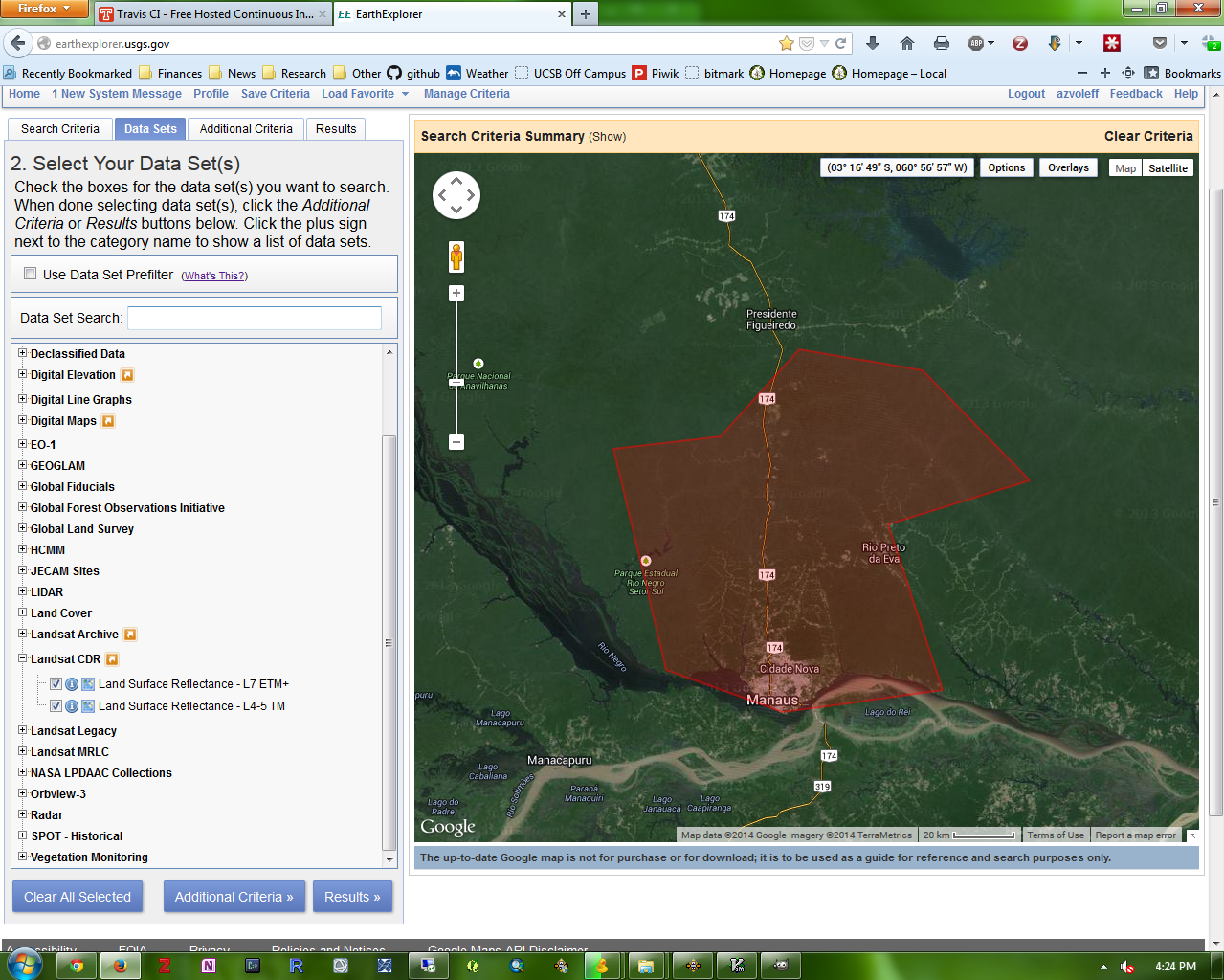
Start by setting up an account on USGS Earth Explorer. After setting up an account, login to the system, and upload a shapefile or draw a polygon to indicate your area of interest. After doing so, click the “Data Sets > >” button on the lower left of the screen. For this example, we will be using Landsat CDR Surface Reflectance imagery. Click the “+” next to “Landsat CDR”, and then click the checkboxes for both “Land Surface Reflectance - L7 ETM+” and also “Land Surface Reflectance - L4-5 TM”:

Now click the “Results > >” button.

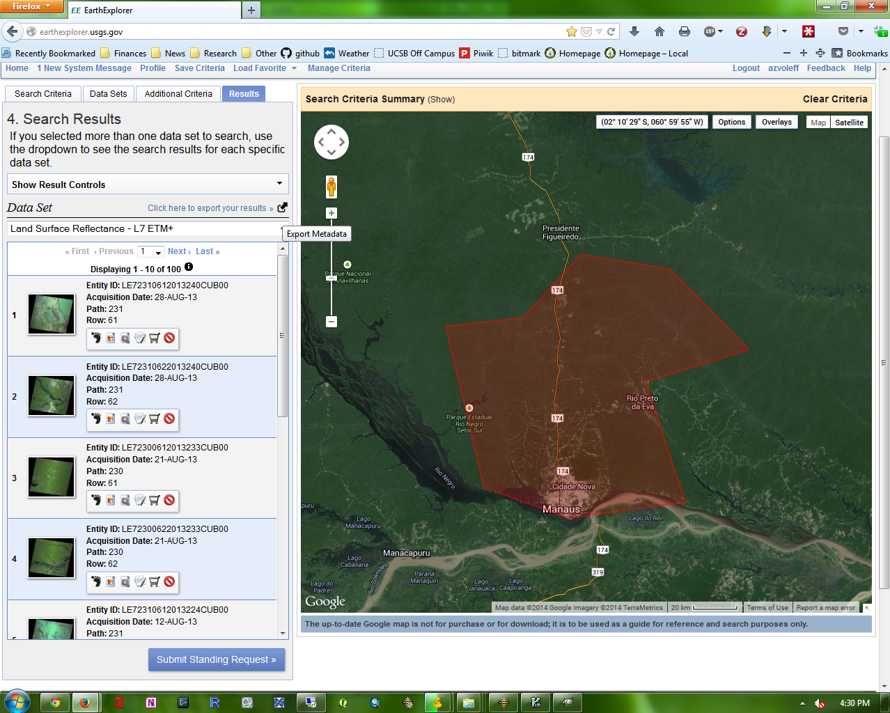
You will now see results for one of the two (Landsat 4-5 and Landsat 7) datasets you selected. Look under “Data Set” on the left side of the screen, and it will say “Land Surface Reflectance - L7 ETM+” if it is displaying the Landsat 7 CDR dataset. You will need to separately export the Landsat 7 and Landsat 4-5 scene lists.

To export the first scene list: from the “Search Results” page, download a CSV file of ALL available Landsat imagery for the search area. To do this, click the “Click here to export your results > >” text near the top right of the screen.

In the “Metadata Export” box, choose “Non-Limited Results” for “Export Type”. For “Format” choose “CSV”:

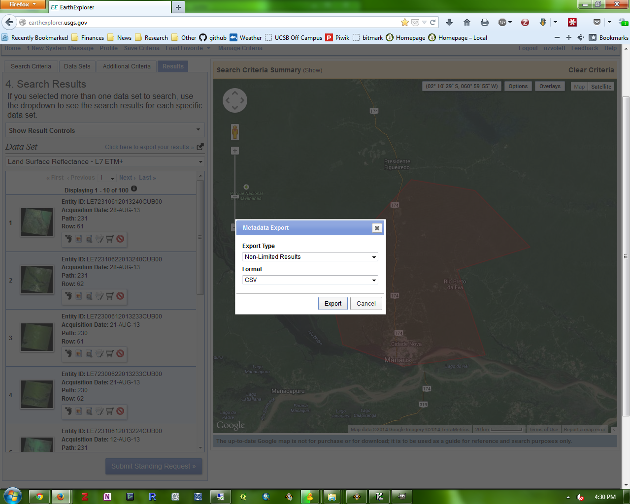
A window will come up saying “Your export file is being generated.” Click “OK”. Repeat the same process for the other CDR dataset, by changing the data set you have selected, and again clicking the “Click here to export your results > >” text.

You will receive two emails at your USGS Earth Explorer registered email address each with a link to one a zipfile containing one of the scene lists. Download these zipfiles and use them for the next step (or use the below example data instead)

Selecting Landsat scenes to download

To follow along with this analysis, download this zipfile with a shapefile of Zone of Interation (ZOI) of the TEAM site in Nam Kading National Protected Area in Lao PDR. The zipfile also includes scene lists from EarthExplorer of all available Landsat scenes (as of April 23, 2014) for this site.

First, read in the Landsat scene lists downloaded from USGS EarthExplorer, using the ee_read function in teamlucc:

l7 <- ee_read('NAK_L7_20140423_scenelist.csv')
l45 <- ee_read('NAK_L4-5_20140423_scenelist.csv')

Now, merge the Landsats 4-5 and Landsat 7 scene lists so they can be analyzed together:

l457 <- merge(l7, l45, all=TRUE)

Selecting Landsat images, particularly for an area covered by multiple Landsat path/rows, can be difficult. The wrspathrow package (available on CRAN) is helpful for producing a quick visualization of the number of Landsat scenes (path/row(s)) needed to cover an area. For example, the below code reads in the ZOI shapefile for Nam Kading, and plots the Landsat path/rows needed to cover the ZOI. This plot uses the path/row polygons included in the wrspathrow package, and includes text labels for each path and row:

library(wrspathrow)
NAK_zoi <- readOGR('.', 'ZOI_NAK_2012_EEsimple')

## OGR data source with driver: ESRI Shapefile 
## Source: ".", layer: "ZOI_NAK_2012_EEsimple"
## with 1 features and 3 fields
## Feature type: wkbPolygon with 2 dimensions

NAK_pathrows <- pathrow_num(NAK_zoi, as_polys=TRUE)
plot(NAK_pathrows)
plot(NAK_zoi, add=TRUE, lty=2, col="#00ff0050")
text(coordinates(NAK_pathrows), labels=paste(NAK_pathrows$PATH, 
                                             NAK_pathrows$ROW, sep=', '))

From the above plots, we can see that it takes scenes from three Landsat path/rows to cover the entire Nam Kading ZOI. Suppose we need images from within a particular period, covering the entire area of that ZOI. The the ee_plot function in the teamlucc package can make a plot of the available imagery within a given time period, color coded by sensor and percent cloud cover. To use this function, first specify a start and end date:

start_date <- as.Date('1995/1/1')
end_date <- as.Date('2000/1/1')

Now use ee_plot to plot the available imagery from within that time period:

ee_plot(l457, start_date, end_date)

Each box in this plot represents a single Landsat scene from the Landsat archive. The color of each box indicates the path and row of that scene, while the outline color of each box indicates the sensor (Landsat 5 versus Landsat 7 for example). The shading of a particular box (light or dark) box indicates the cloud cover of that scene (lighter colors correspond to scenes with greater cloud cover).

From this plot, we can see that within the 1995 to 2000 time period, January 1996 is the only month in which images are available for all three path/rows needed to cover the Nam Kading ZOI. Further, from the shading of the boxes in that month, we can tell that these images are almost cloud free, and are from Landsat 5 (indicated by the green outlines).

Note that ee_plot will by default only plot imagery where greater than 70% of the image is unobscured by plots (i.e. less than 30% cloud cover). This default can be changed by supplying the min_clear parameter to ee_plot.

When dealing with a large number of scenes, a different type of plot can be helpful. The normalize argument to ee_plot tells ee_plot to calculate the best (lowest cloud cover) image for each path and row for each month. Then, ee_plot sums across all the path and rows, and plots the results:

ee_plot(l457, start_date, end_date, normalize=TRUE)

This type of plot is helpful in visualizing the periods in which the greatest proportion of a site can be covered by cloud-free (or nearly cloud-free) imagery.

Downloading Landsat scenes using ESPA

teamlucc also facilitates placing orders for imagery using the USGS ESPA system. The ESPA system accepts scenes lists as a text file. To output a scene list for upload to ESPA, use the espa_scenelist function, specifying the start and end dates needed, and the name of the output file:

espa_scenelist(l457, as.Date('1996/1/1'), as.Date('1996/12/31'), 
               'NAK_ESPA_scenelist_1986.txt')

The above line of code will save a text file named NAK_ESPA_scenelist_1986.txt in your current working directory. To place an order, login to the ESPA system, and upload the text file.

After receiving an email from the ESPA system notifying you that your order is processed, download the order from within R using the espa_download function by specifying 1) the email address you used to place the order, 2) the ESPA order ID number (included in the email from ESPA), and 3) the output folder in which to save the downloaded images. espa_download will first check within the specified output folder to see if each image already exists, and will not re-download existing files unless the existing files do not match the files available on ESPA.

Note the below code is not working as of 7/1/2014 due to changes in the ESPA download system. I will update this post when the code is working again.

espa_download('azvoleff@example.com', '272014-114611', 'D:/ESPA_Downloads')

## Error in espa_download("azvoleff@example.com", "272014-114611", "D:/ESPA_Downloads"): Due to changes in the ESPA system, espa_download is not working as of 7/1/2014