Overview
This post outlines how to use the teamlucc package to preprocess imagery from
the Landsat Surface Reflectance Climate Data Record
(CDR) archive. The teamlucc package
supports a number of common preprocessing steps, including:
- Conversion of CDR files to any GDAL supported file format
- Cropping Landsat tiles to a given area of interest (AOI)
- Mosaicking and cropping of DEM tiles (such as ASTER or SRTM) to a given AOI or Landsat path/row
- Topographic correction of CDR scenes
Getting started
First load the teamlucc package, and the rgdal package:
library(teamlucc)## Loading required package: Rcpp
## Loading required package: raster
## Loading required package: sp## Warning: replacing previous import by 'raster::buffer' when loading
## 'teamlucc'## Warning: replacing previous import by 'raster::interpolate' when loading
## 'teamlucc'## Warning: replacing previous import by 'raster::rotated' when loading
## 'teamlucc'library(rgdal)## rgdal: version: 0.9-1, (SVN revision 518)
## Geospatial Data Abstraction Library extensions to R successfully loaded
## Loaded GDAL runtime: GDAL 1.11.0, released 2014/04/16
## Path to GDAL shared files: C:/Users/azvoleff/R/win-library/3.1/rgdal/gdal
## GDAL does not use iconv for recoding strings.
## Loaded PROJ.4 runtime: Rel. 4.8.0, 6 March 2012, [PJ_VERSION: 480]
## Path to PROJ.4 shared files: C:/Users/azvoleff/R/win-library/3.1/rgdal/projDEM setup
Before CDR surface reflectance images can be topographically corrected with
teamlucc, a digital elevation model (DEM) needs to be obtained that is in the
same resolution and coordinate system as the CDR imagery, and slope and aspect
need to be calculated. The auto_setup_dem function in the teamlucc package
facilitates this task. There are many options you can supply to
auto_setup_dem - see ?auto_setup_dem for more information on these options.
If you do not want to topographically correct your imagery, you can skip this
step and move ahead to the next section.
auto_setup_dem assembles a DEM to cover a given area of interest (AOI), and
can mosaic multiple DEM files if needed to cover an AOI. To use
auto_setup_dem, the user must first define the area of interest with an AOI
polygon. If you have a shapefile of an area of interest, load it into R using
the readOGR command. The readOGR command needs the folder the shapefile is
in (in this example the current working directory, specified by .) as the
first parameter, and the filename of the shapefile (without the “.shp”
extension) as the second parameter (PA_VB) in this example). This example
uses a shapefile of the boundary of the Braulio Carrillo National Park, in
which the Volcán Barva TEAM
site is located:
aoi <- readOGR('.', 'PA_VB')## OGR data source with driver: ESRI Shapefile
## Source: ".", layer: "PA_VB"
## with 5 features and 8 fields
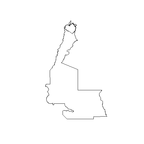
## Feature type: wkbPolygon with 2 dimensionsplot(aoi)
As seen in the above plot, there are a number of adjoining polygons in this
shapefile. The functions in teamlucc expect the AOI to be of length one. So
calculate the convex hull of the AOI using the functions in the rgeos
package:
library(rgeos)## rgeos version: 0.3-8, (SVN revision 460)
## GEOS runtime version: 3.4.2-CAPI-1.8.2 r3921
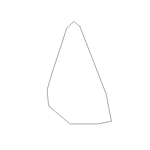
## Polygon checking: TRUEaoi <- gConvexHull(aoi)The AOI is now a single polygon:
plot(aoi)
If you do not have an AOI, but know the Landsat path and row you want to work
with, an alternative is to define the AOI based on the path and row, using the
wrspathrow R package, and supplying the desired path and row numbers. Here
127 is the WRS-2 path number, and 47 is the WRS-2 row number for the
path/row at the center of the above AOI:
library(wrspathrow)
aoi_from_pathrow <- pathrow_poly(127, 47)
In addition to the AOI, auto_setup_dem needs to know the location and spatial
extents of the DEM files you have available on your machine. This list can be
assembled automatically using the get_extent_polys function in teamlucc.
See ?get_extent_polys for more information. The below code will fail on your
machine because you will not have the proper DEMs for this example. Download
the proper DEMs for the area in which you are working and place them in a
folder on your machine if you want to test this function.
dem_files <- dir('H:/Data/CGIAR_SRTM/Tiles', pattern='.tif$', full.names=TRUE)
dems <- lapply(dem_files, raster)
dem_extents <- get_extent_polys(dems)
For flexibility, auto_setup_dem can optionally crop each output DEM to the
spatial extent of the supplied AOI. If crop_to_aoi=TRUE, then
auto_setup_dem will crop the DEMs to the spatial extent of the supplied AOI.
If crop_to_aoi=FALSE, then auto_setup_dem will crop the DEMs to the extent
of the Landsat path/rows needed to cover the AOI.
Lastly, auto_setup_dem needs to know where to save its output. For this
example, save the output to the current working directory .. Now that all of
the essential inputs are defined, auto_setup_dem can be called:
auto_setup_dem(aoi, '.', dem_extents, crop_to_aoi=TRUE)## [1] "2014-11-13 16:49:49: started \"Processing DEMS for 1 path/rows\""
## [1] "2014-11-13 16:49:50: started \"Processing 1 of 1: 015-053\""
## [1] "2014-11-13 16:50:00: finished \"Processing 1 of 1: 015-053\" (10.047s elapsed)"
## [1] "2014-11-13 16:50:00: finished \"Processing DEMS for 1 path/rows\" (10.285s elapsed)"The result will be a mosaicked DEM, in the current working directory, that can
be used for topographically correcting imagery with the
auto_preprocess_landsat function.
Preprocessing
Images are delivered from the CDR archive in either ENVI format, GeoTIFF
format, or Hierarchical Data Format (HDF). The teamlucc package will, by
default, convert HDF or ENVI format images to a GeoTIFF format, as these image
files can be easily read in R and in most commonly used remote sensing and GIS
software packages. This example assumes you want GeoTIFF output - see the help
files for teamlucc for other output options.
First you will need to acquire a time series of CDR imagery for your site. The
espa_download function can facilitate downloading files from an ESPA order.
Also see the post on Filtering and downloading Landsat
scenes for more details on how
teamlucc can help with image acquisition.
Once you have downloaded your imagery from ESPA, I recommend you put all of the
zip files from your download in a single folder. You can then use the
teamlucc espa_extract function to automate extracting your CDR image files,
including placing the extracted files in consistently named output folders.
If, for example, your files are located in espa_downloads and you want to
extract them to espa_extracts, run the following (this block, and the next
block of code, will both fail on your computer since you do not have the
required imagery - this is only an example, download your own imagery to follow
along):
download_folder <- 'espa_downloads'
extract_folder <- 'espa_extracts'
espa_extract(download_folder, extract_folder)
## 1 of 2. Extracting LT50150532000044-SC20140514195145.tar.gz to espa_extracts/015-053_2000-044_LT5
## 2 of 2. Extracting LT50150532001014-SC20140514195632.tar.gz to espa_extracts/015-053_2001-014_LT5Now that the CDR format image files are extracted, you are ready to run
auto_preprocess_landsat. As with auto_setup_dem, there are many options you
can supply to auto_preprocess_landsat - see ?auto_preprocess_landsat. The
below is a simple example of how to call auto_preprocess_landsat.
The image_dirs line below is just a fancy way of finding all the folders
located in extract_folder that contain CDR imagery. You could just as easily
specify these folders individually as as a list of strings, like: image_dirs
<- c('C:/folder1', 'C:/folder2') if you had two CDR Landsat scenes located in
C:/folder1 and C:/folder2, respectively.
The prefix parameter specifies a string that will be used in naming files
output by auto_preprocess_landsat. For prefix I suggest you use a short (2
or 3 character) site name or site code that is meaningful to you.
There are two other options we provide below to auto_preprocess_landsat.
tc=TRUE tells auto_preprocess_landsat to perform topographic correction.
Because of this, we also need to specify dem_path (where the DEM files
preprocessed by auto_setup_dem are located), so that the DEM files for this
scene can be found. Here we set dem_path='.' as the DEM is in our current
working directory. We supply an AOI (same AOI as above) to crop the output
images. verbose=TRUE indicates that we want detailed progress messages to
print while the script is running. The output of auto_preprocess_landsat is a
data.frame with a list of the preprocessed files and their file formats.
image_dirs <- dir('espa_extracts',
                  pattern='^[0-9]{3}-[0-9]{3}_[0-9]{4}-[0-9]{3}_((LT[45])|(LE7))$',
                  full.names=TRUE)
filelist <- auto_preprocess_landsat(image_dirs, prefix='VB', tc=TRUE,
                                    dem_path='.', aoi=aoi, verbose=TRUE)
## Warning: executing %dopar% sequentially: no parallel backend registered## [1] "2014-11-13 16:50:52: started \"Preprocessing 015-053_2000-044_L5TSR\""
## [1] "2014-11-13 16:50:52: started \"cropping and reprojecting\""## Warning in build_mask_vrt(file_base, mask_vrt_file, file_format): Using
## "fmask_band" instead of newer "cfmask_band" band name## [1] "2014-11-13 16:51:03: finished \"cropping and reprojecting\" (10.787s elapsed)"
## [1] "2014-11-13 16:51:03: started \"topocorr\""
## [1] "2014-11-13 16:53:25: finished \"topocorr\" (142.071s (~2.37 minutes) elapsed)"
## [1] "2014-11-13 16:53:25: started \"writing data\""
## [1] "2014-11-13 16:53:29: finished \"writing data\" (4.052s elapsed)"
## [1] "2014-11-13 16:53:29: finished \"Preprocessing 015-053_2000-044_L5TSR\" (156.919s (~2.62 minutes) elapsed)"
## [1] "2014-11-13 16:53:30: started \"Preprocessing 015-053_2001-014_L5TSR\""
## [1] "2014-11-13 16:53:30: started \"cropping and reprojecting\""## Warning in build_mask_vrt(file_base, mask_vrt_file, file_format): Using
## "fmask_band" instead of newer "cfmask_band" band name## [1] "2014-11-13 16:53:44: finished \"cropping and reprojecting\" (14.161s elapsed)"
## [1] "2014-11-13 16:53:44: started \"topocorr\""
## [1] "2014-11-13 16:55:55: finished \"topocorr\" (131.256s (~2.19 minutes) elapsed)"
## [1] "2014-11-13 16:55:55: started \"writing data\""
## [1] "2014-11-13 16:55:59: finished \"writing data\" (4.236s elapsed)"
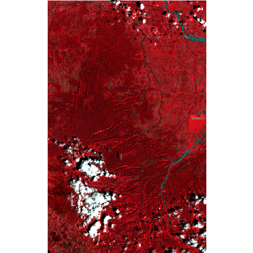
## [1] "2014-11-13 16:55:59: finished \"Preprocessing 015-053_2001-014_L5TSR\" (149.662s (~2.49 minutes) elapsed)"The result is two cropped, reprojected, and topographically corrected Landsat images covering the specified AOI. One image from 2000:
ls_2000 <-  brick('espa_extracts/015-053_2000-044_LT5/VB_015-053_2000-044_L5TSR_tc.tif')
ls_2000 <- linear_stretch(ls_2000, pct=2, max_val=255)
browse_image(ls_2000, r=4, g=3, b=2)
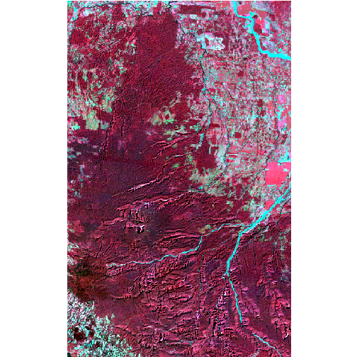
And one image from 2001:
ls_2001 <- brick('espa_extracts/015-053_2001-014_LT5/VB_015-053_2001-014_L5TSR_tc.tif')
ls_2001 <- linear_stretch(ls_2001, pct=2, max_val=255)
browse_image(ls_2001, r=4, g=3, b=2)
There is a fair amount of cloud cover in the 2000 image. See the post on cloud removal for one means of addressing this issue.
